Note
Go to the end to download the full example code.
Exporting pyAFQ Results#
This example shows how to use the export methods to obtain results from
the ParticipantAFQ object. The export methods are used to calculate
derived quantities from the data, such as DTI parameters, tract profiles,
and bundle segmentations.
import os
import os.path as op
import plotly
from AFQ.api.participant import ParticipantAFQ
import AFQ.data.fetch as afd
Preparing the ParticipantAFQ object#
In this example, we will create a ParticipantAFQ object based on the Getting started with pyAFQ - ParticipantAFQ example. Please refer to that example for a detailed description of the parameters.
afd.organize_stanford_data(clear_previous_afq="track")
data_dir = op.join(afd.afq_home, "stanford_hardi", "derivatives", "vistasoft",
"sub-01", "ses-01", "dwi")
dwi_data_file = op.join(data_dir, "sub-01_ses-01_dwi.nii.gz")
bval_file = op.join(data_dir, "sub-01_ses-01_dwi.bval")
bvec_file = op.join(data_dir, "sub-01_ses-01_dwi.bvec")
output_dir = op.join(afd.afq_home, "stanford_hardi",
"derivatives", "afq", "sub-01")
os.makedirs(output_dir, exist_ok=True)
# Initialize the ParticipantAFQ object
myafq = ParticipantAFQ(
dwi_data_file=dwi_data_file,
bval_file=bval_file,
bvec_file=bvec_file,
output_dir=output_dir,
tracking_params={
"n_seeds": 25000,
"random_seeds": True,
"rng_seed": 2022,
"trx": True,
"num_chunks": True
},
)
The Export Method#
The ParticipantAFQ object has a method called export, which allows the user
to calculate various derived quantities from the data.
The export method can be called with a string argument that specifies the
type of quantity to be calculated. For example, myafq.export("OPTIONS").
To list the available options, you can call the export method with the
argument “help”. This will return a list of all the available options for
the export method.
myafq.export("help")
Here is a list of valid attributes to export: dict_keys(['dwi_data_file', 'bval_file', 'bvec_file', 'output_dir', 'best_scalar', 'base_fname', 'data', 'gtab', 'dwi', 'dwi_affine', 'min_bval', 'max_bval', 'filter_b', 'b0_threshold', 'b0', 'masked_b0', 'dti_tf', 'dti_params', 'robust_tensor_fitting', 'fwdti_tf', 'fwdti_params', 'dki_tf', 'dki_params', 'msdki_tf', 'msdki_params', 'msdki_msd', 'msdki_msk', 'csd_params', 'csd_response', 'csd_sh_order_max', 'csd_lambda_', 'csd_tau', 'csd_fa_thr', 'csd_pmap', 'csd_ai', 'gq_params', 'gq_iso', 'gq_aso', 'gq_sampling_length', 'gq_pmap', 'gq_ai', 'rumba_model', 'rumba_wm_response', 'rumba_gm_response', 'rumba_csf_response', 'rumba_n_iter', 'rumba_params', 'rumba_fit', 'rumba_f_csf', 'rumba_f_gm', 'rumba_f_wm', 'opdt_params', 'opdt_gfa', 'opdt_sh_order', 'opdt_pmap', 'opdt_ai', 'csa_params', 'csa_gfa', 'csa_sh_order', 'csa_pmap', 'csa_ai', 'fwdti_fa', 'fwdti_md', 'fwdti_fwf', 'dti_fa', 'dti_lt0', 'dti_lt1', 'dti_lt2', 'dti_lt3', 'dti_lt4', 'dti_lt5', 'dti_cfa', 'dti_pdd', 'dti_md', 'dti_ga', 'dti_rd', 'dti_ad', 'dki_kt0', 'dki_kt1', 'dki_kt2', 'dki_kt3', 'dki_kt4', 'dki_kt5', 'dki_kt6', 'dki_kt7', 'dki_kt8', 'dki_kt9', 'dki_kt10', 'dki_kt11', 'dki_kt12', 'dki_kt13', 'dki_kt14', 'dki_lt0', 'dki_lt1', 'dki_lt2', 'dki_lt3', 'dki_lt4', 'dki_lt5', 'dki_fa', 'dki_md', 'dki_awf', 'sphere', 'gtol', 'dki_mk', 'dki_kfa', 'dki_ga', 'dki_rd', 'dki_ad', 'dki_rk', 'dki_ak', 'brain_mask', 'brain_mask_definition', 'bundle_dict', 'reg_template', 'tmpl_name', 'bundle_info', 'reg_template_spec', 'reg_template_space_name', 'b0_warped', 'template_xform', 'rois', 'mapping', 'mapping_definition', 'reg_subject', 'reg_subject_spec', 'bundles', 'segmentation_params', 'indiv_bundles', 'sl_counts', 'median_bundle_lengths', 'density_maps', 'profiles', 'profile_weights', 'n_points_profile', 'scalar_dict', 'scalars', 'seed', 'seed_thresh', 'stop', 'stop_thresh', 'streamlines', 'tracking_params', 'fodf', 'import_tract', 'tractography_ngpus', 'chunk_size', 'all_bundles_figure', 'sbv_lims_bundles', 'volume_opacity_bundles', 'n_points_bundles', 'indiv_bundles_figures', 'sbv_lims_indiv', 'volume_opacity_indiv', 'n_points_indiv', 'tract_profile_plots', 'viz_backend', 'virtual_frame_buffer', 'viz_backend_spec'])
Note
No all options are possible even if they are valid. This will depend on you dataset and pyAFQ API parameters. For example, you cannot calculate DKI model from single shell data. Please refer to Tractography Parameters for more documentation.
Calculating DTI FA (Diffusion Tensor Imaging Fractional Anisotropy)#
FA can be computed using the DTI model, by explicitly calling
myafq.export("dti_fa"). This triggers the computation of DTI parameters,
and stores the results in the AFQ derivatives directory. In addition, it
calculates the FA from these parameters and stores it in a different file in
the same directory.
Note
The AFQ API computes quantities lazily. This means that DTI parameters are not computed until they are required. This means that the first line below is the one that requires time.
The result of the call to export is the filename of the corresponding FA
files.
FA_fname = myafq.export("dti_fa")
Recognizing the bundles and calculating tract profiles:#
Typically, users of pyAFQ are interested in calculating not only an overall
map of the FA, but also the major white matter pathways (or bundles) and
tract profiles of tissue properties along their length. To trigger the
pyAFQ pipeline that calculates the profiles, users can call the
export("profiles") method:
Note
Running the code below triggers the full pipeline of operations leading to the computation of the tract profiles. Therefore, it takes a little while to run (about 40 minutes, typically).
myafq.export("profiles")
'/home/runner/AFQ_data/stanford_hardi/derivatives/afq/sub-01/sub-01_ses-01_desc-profiles_tractography.csv'
Visualizing the bundles and calculating tract profiles:#
The pyAFQ API provides several ways to visualize bundles and profiles.
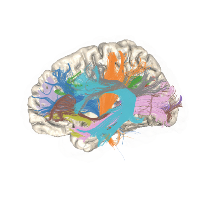
First, we will run a function that exports an html file that contains an interactive visualization of the bundles that are segmented.
Note
By default we resample a 100 points within a bundle, however to reduce processing time we will only resample 50 points.
Once it is done running, it should pop a browser window open and let you interact with the bundles.
Note
You can hide or show a bundle by clicking the legend, or select a single bundle by double clicking the legend. The interactive visualization will also all you to pan, zoom, and rotate.
bundle_html = myafq.export("all_bundles_figure")
plotly.io.show(bundle_html[0])
