Changing model flexibility

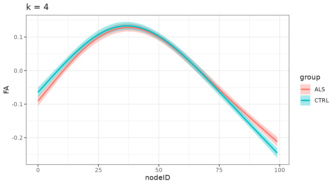
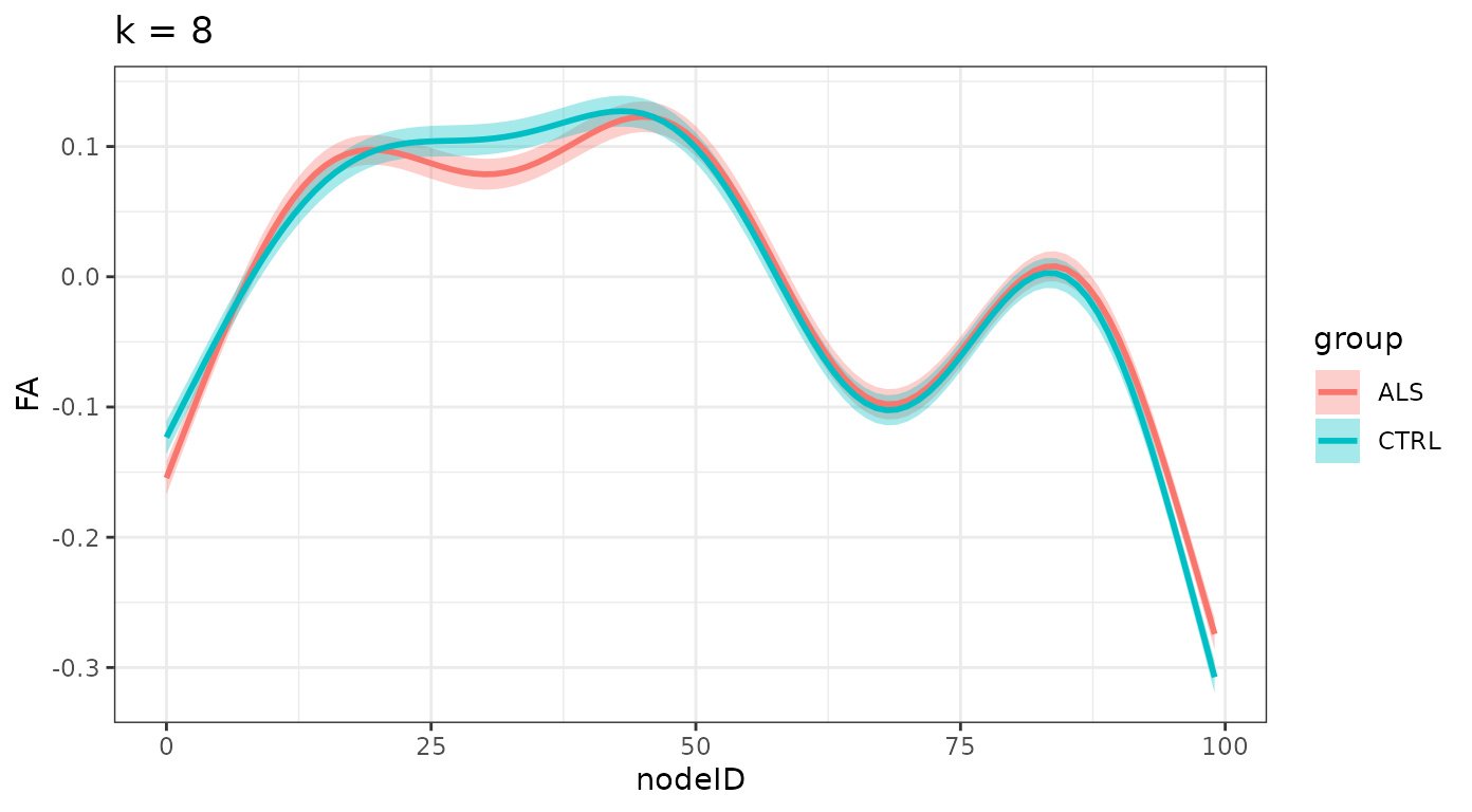
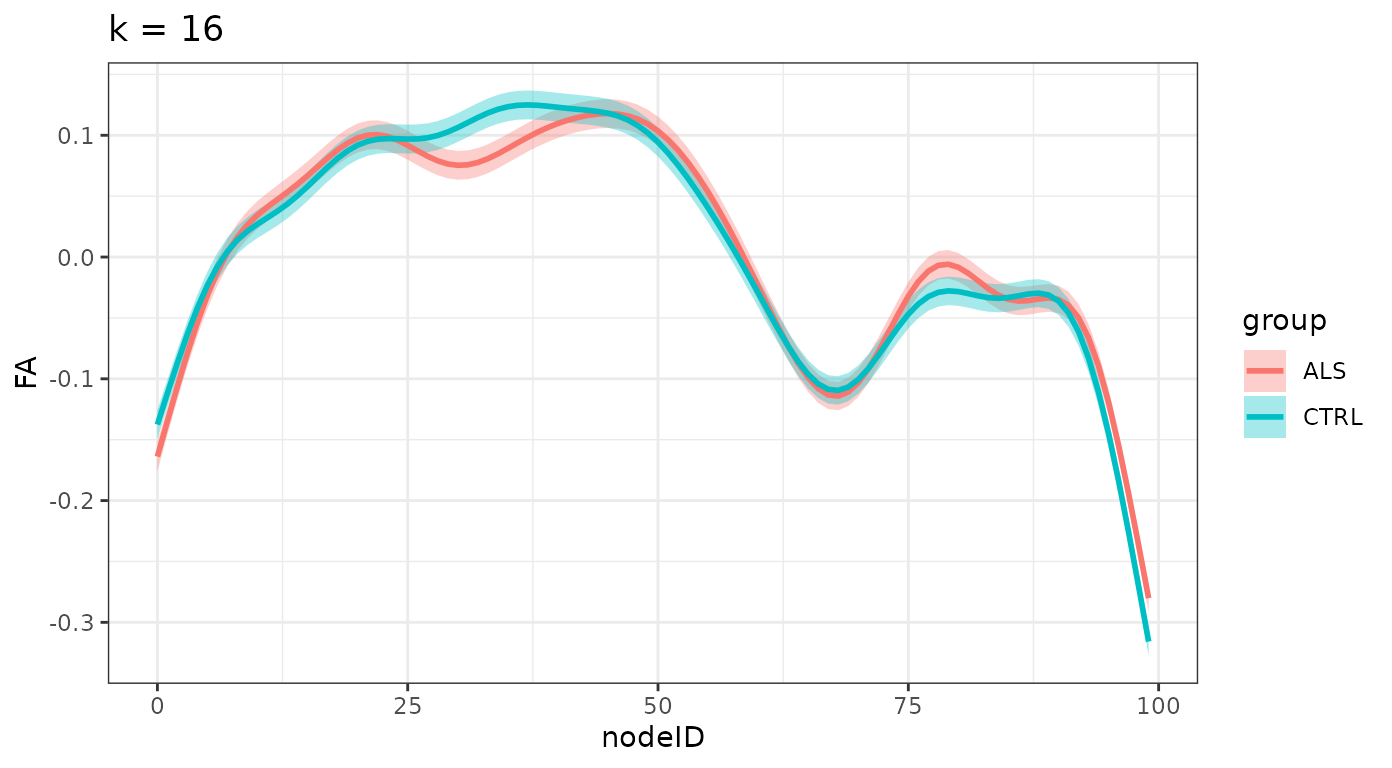
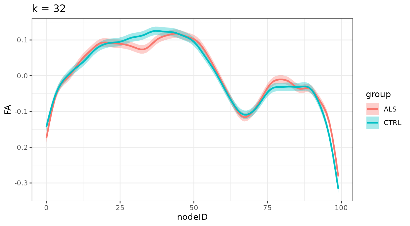
This vignette demonstrates how a GAM model changes with increased flexibility.

The data we will use here contains tract profiles from diffusion MRI measurements in a group of patients with Amyotrophic Lateral Sclerosis (ALS) and a group of matched controls (Sarica et al. 2017).

We start by loading the tractable library and gratia, as well as ggplot2, which we will use to interpret the fitted model.

library(tractable)
library(gratia)
library(ggplot2)

Next, we will use a function that is included in tractable to read this dataset directly into memory.

Importantly, both the group (“ALS” or “CTRL”) and the subject identifier (“subjectID”) need to be factors for subsequent analysis to work properly.

df_sarica <- read_afq_sarica(na_omit = TRUE) 
df_sarica
#> # A tibble: 93,377 × 8
#>    subjectID   tractID                 nodeID    fa    md   age group gender
#>    <fct>       <chr>                    <dbl> <dbl> <dbl> <dbl> <fct> <fct> 
#>  1 subject_000 Left Thalamic Radiation      0 0.174 0.965    54 ALS   F     
#>  2 subject_000 Left Thalamic Radiation      1 0.227 0.912    54 ALS   F     
#>  3 subject_000 Left Thalamic Radiation      2 0.282 0.874    54 ALS   F     
#>  4 subject_000 Left Thalamic Radiation      3 0.318 0.851    54 ALS   F     
#>  5 subject_000 Left Thalamic Radiation      4 0.341 0.830    54 ALS   F     
#>  6 subject_000 Left Thalamic Radiation      5 0.353 0.812    54 ALS   F     
#>  7 subject_000 Left Thalamic Radiation      6 0.357 0.802    54 ALS   F     
#>  8 subject_000 Left Thalamic Radiation      7 0.357 0.795    54 ALS   F     
#>  9 subject_000 Left Thalamic Radiation      8 0.359 0.790    54 ALS   F     
#> 10 subject_000 Left Thalamic Radiation      9 0.371 0.784    54 ALS   F     
#> # ℹ 93,367 more rows

We fit models with different levels of flexibility, encoded in different values of k:

k_values <- c(4, 8, 16, 32)

models <- list()
for (i in 1:length(k_values)){
   models[[i]] <- tractable_single_tract(
    target     = "fa", 
    df         = df_sarica, 
    tract      = "Right Corticospinal",
    regressors = c("age", "group"), 
    node_k     = k_values[i], 
    node_group = "group"
  )
}

And we plot the smooths, divided by group for each one of these levels:

plots <- list()
for (i in 1:length(k_values)){
  plots[[i]] <- models[[i]] %>%
    smooth_estimates() %>%
    add_confint() %>%
    dplyr::filter(.type != "Random effect") %>%
    ggplot(aes(x = nodeID, y = .estimate, ymin = .lower_ci, 
               ymax = .upper_ci, group = group, color = group, 
               fill = group)) +
    geom_ribbon(color = NA, alpha = 0.35) + 
    geom_line(linewidth = 1) +
    scale_y_continuous(name = "FA") +
    ggtitle(sprintf("k = %d", k_values[i])) + 
    theme_bw()
}
names(plots) <- sprintf("k = %d", k_values)

plots
#> $`k = 4`

#> 
#> $`k = 8`

#> 
#> $`k = 16`

#> 
#> $`k = 32`

References

Sarica, Alessia, Antonio Cerasa, Paola Valentino, Jason Yeatman, Maria Trotta, Stefania Barone, Alfredo Granata, et al. 2017. “The Corticospinal Tract Profile in Amyotrophic Lateral Sclerosis.” Hum. Brain Mapp. 38 (2): 727–39.