Use parametric statistics for group comparison

As a contrast to the approach presented in other examples, we also present a more “standard” statistical approach to analyze tract profile data. Here, we will conduct a point-by-point group comparison using a linear model fit using the standard ordinary least squares (OLS) method.

This example first fetches the ALS classification dataset from Sarica et al [1]. This dataset contains tractometry features from 24 patients with ALS and 24 demographically matched control subjects. It then uses the statsmodels library to compare between the tract profiles of the two groups in one tract (the left corticospinal tract) and in one feature (FA).

[1]

Alessia Sarica, et al. “The Corticospinal Tract Profile in AmyotrophicLateral Sclerosis” Human Brain Mapping, vol. 38, pp. 727-739, 2017 DOI: 10.1002/hbm.23412

import matplotlib.pyplot as plt

from afqinsight import AFQDataset
from afqinsight.parametric import node_wise_regression
from afqinsight.plot import plot_regression_profiles

Fetch data from Sarica et al.

As a shortcut, we have incorporated a few studies into the software. In these cases, a AFQDataset class instance can be initialized using the AFQDataset.from_study() static method. This expects the name of one of the studies that are supported (see the method documentation for the list of these studies). By passing “sarica”, we request that the software download the data from this study and initialize an object for us from this data.

afqdata = AFQDataset.from_study("sarica")

# Specify the tracts of interest
# ------------------------------
# Many times we have a specific set of tracts we want to analyze. We can specify
# those tracts using a list with each tract of interest

tracts = ["Left Arcuate", "Right Arcuate", "Left Corticospinal", "Right Corticospinal"]

# Set up plot, run linear models, and show the results
# ----------------------------------------------------
# With the next few lines of code, we fit a linear model in order to predict
# group differences in the diffusion properties of our tracts of interest. The
# function `node_wise_regression` does this by looping through each node of a
# tract and predicting our diffusion metric, in this case FA, as a function of
# group. The initializer `OLS.from_formula` takes `R-style formulas
# <https://www.statsmodels.org/dev/example_formulas.html>`_ as its model specification.
# Here, we are using the `"group"` variable as a categorical variable in the model.
# We can also specify linear-mixed effects models for more complex phenotypic data
# by passing in the appropriate model formula and setting `lme=True`.
#
# Because we conducted 100 comparisons, we need to correct the p-values that
# we obtained for the potential for a false discovery. There are multiple
# ways to conduct multiple comparison correction, and we will not get into
# the considerations in selecting a method here. The function `node_wise_regression`
# uses Benjamini/Hochberg FDR controlling method. This returns a boolean array for
# the p-values that are rejected at a specified alpha level (after correction),
# as well as an array of the corrected p-values.

num_cols = 2

# Define the figure and grid
fig, axes = plt.subplots(nrows=2, ncols=num_cols, figsize=(10, 6))


# Loop through the data and generate plots
for i, tract in enumerate(tracts):
    # fit node-wise regression for each tract based on model formula
    tract_dict = node_wise_regression(afqdata, tract, "fa", "fa ~ C(group)")

    row = i // num_cols
    col = i % num_cols

    axes[row][col].set_title(tract)

    # Visualize
    # ----------
    # We can visualize the results with the `plot_regression_profiles`
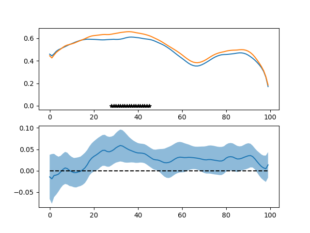
    # function. Each subplot shows the tract profiles of the two groups,
    # while controlling for any covariates, with stars indicating the nodes
    # at which the null hypothesis is rejected.

    plot_regression_profiles(tract_dict, axes[row][col])

# Adjust layout to prevent overlap
plt.tight_layout()

# Show the plot
plt.show()

subjects.csv:   0%|          | 0.00/515 [00:00<?, ?iB/s]
subjects.csv: 1.56kiB [00:00, 5.66MiB/s]

nodes.csv:   0%|          | 0.00/5.14M [00:00<?, ?iB/s]
nodes.csv: 7.52MiB [00:00, 75.2MiB/s]
nodes.csv: 13.5MiB [00:00, 80.0MiB/s]
/opt/hostedtoolcache/Python/3.12.8/x64/lib/python3.12/site-packages/afqinsight/transform.py:144: FutureWarning: The previous implementation of stack is deprecated and will be removed in a future version of pandas. See the What's New notes for pandas 2.1.0 for details. Specify future_stack=True to adopt the new implementation and silence this warning.
  features = interpolated.stack(["subjectID", "tractID", "metric"]).unstack(