Classify ALS diagnosis from white matter features#

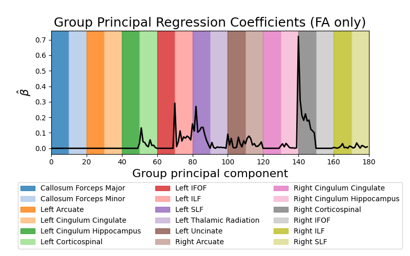
Predict ALS diagnosis from white matter features. This example fetches the ALS classification dataset from Sarica et al [1]. This dataset contains tractometry features from 24 patients with ALS and 24 demographically matched control subjects. The plots display the absolute value of the mean regression coefficients (averaged across cross-validation splits) for the fractional anisotropy (FA) features.

To save computational time, we take the first 10 principal components from each feature group (i.e. from each metric-bundle combination). For more details on this approach in a research setting, please see [2].

import matplotlib.pyplot as plt
import numpy as np
from groupyr.decomposition import GroupPCA
from sklearn.impute import SimpleImputer
from sklearn.model_selection import cross_validate

from afqinsight import AFQDataset, make_afq_classifier_pipeline

Fetch data from Sarica et al.#

As a shortcut, we have incorporated a few studies into the software. In these cases, a AFQDataset class instance can be initialized using the AFQDataset.from_study() static method. This expects the name of one of the studies that are supported (see the method documentation for the list of these studies). By passing “sarica”, we request that the software download the data from this study and initialize an object for us from this data.

afqdata = AFQDataset.from_study("sarica")

# Examine the data
# ----------------
# ``afqdata`` is an ``AFQDataset`` object, with properties corresponding to
# the tractometry features and phenotypic targets.

X = afqdata.X
y = afqdata.y.astype(float)  # SGL expects float targets
groups = afqdata.groups
feature_names = afqdata.feature_names
group_names = afqdata.group_names
subjects = afqdata.subjects

# Reduce data dimensionality
# --------------------------
# Here we reduce computation time by taking the first 10 principal components of
# each feature group and performing SGL logistic regression on those components.
# If you want to train an SGL model without group PCA, set ``do_group_pca =
# False``. This will increase the number of features by an order of magnitude
# and slow down execution time.

do_group_pca = True

if do_group_pca:
    n_components = 10

    # The next three lines retrieve the group structure of the group-wise PCA
    # and store it in ``groups_pca``. We do not use the imputer or GroupPCA transformer
    # for anything else
    imputer = SimpleImputer(strategy="median")
    gpca = GroupPCA(n_components=n_components, groups=groups)
    groups_pca = gpca.fit(imputer.fit_transform(X)).groups_out_

    transformer = GroupPCA
    transformer_kwargs = {"groups": groups, "n_components": n_components}
else:
    transformer = False
    transformer_kwargs = None


# Create the classification pipeline
# ----------------------------------
# The core computational machinery is a pipeline. These operate as scikit-learn
# compatible pipelines, so we can pass them to scikit-learn functions.
# There are many options that need to be set to configure the pipeline object.

pipe = make_afq_classifier_pipeline(
    imputer_kwargs={"strategy": "median"},  # Use median imputation
    use_cv_estimator=True,  # Automatically determine the best hyperparameters
    feature_transformer=transformer,  # See note above about group PCA
    feature_transformer_kwargs=transformer_kwargs,
    scaler="standard",  # Standard scale the features before regression
    groups=(
        groups_pca if do_group_pca else groups
    ),  # SGL will use the original feature groups or the PCA feature groups depending on the choice above # noqa E501
    verbose=0,  # Be quiet!
    pipeline_verbosity=False,  # No really, be quiet!
    tuning_strategy="bayes",  # Use BayesSearchCV to determine optimal hyperparameters
    n_bayes_iter=20,  # Consider only this many points in hyperparameter space
    cv=3,  # Use three CV splits to evaluate each hyperparameter combination
    l1_ratio=[0.0, 1.0],  # Explore the entire range of ``l1_ratio``
    eps=5e-2,  # This is the ratio of the smallest to largest ``alpha`` value
    tol=1e-2,  # Set a lenient convergence tolerance just for this example
)

# Fit and cross-validate
# ----------------------
# The ``pipe`` object is a scikit-learn pipeline and can be used in other
# scikit-learn functions

scores = cross_validate(
    pipe, X, y, cv=5, return_train_score=True, return_estimator=True
)

# Display results
# ---------------

print(f"Mean train score: {np.mean(scores['train_score']):5.3f}")
print(f"Mean test score:  {np.mean(scores['test_score']):5.3f}")
print(f"Mean fit time:    {np.mean(scores['fit_time']):5.2f}s")
print(f"Mean score time:  {np.mean(scores['score_time']):5.2f}s")

mean_coefs = np.mean(
    np.abs([est.named_steps["estimate"].coef_ for est in scores["estimator"]]), axis=0
)

fig, ax = plt.subplots(1, 1, figsize=(8, 5))
_ = ax.plot(mean_coefs[:180], color="black", lw=2)
_ = ax.set_xlim(0, 180)

colors = plt.get_cmap("tab20").colors
for grp, grp_name, color in zip(groups_pca[:18], group_names, colors):
    _ = ax.axvspan(grp.min(), grp.max() + 1, color=color, alpha=0.8, label=grp_name[1])

box = ax.get_position()
_ = ax.set_position(
    [box.x0, box.y0 + box.height * 0.375, box.width, box.height * 0.625]
)

_ = ax.legend(loc="upper center", bbox_to_anchor=(0.5, -0.2), ncol=3)
_ = ax.set_ylabel(r"$\hat{\beta}$", fontsize=16)
_ = ax.set_xlabel("Group principal component", fontsize=16)
_ = ax.set_title("Group Principal Regression Coefficients (FA only)", fontsize=18)

Group Principal Regression Coefficients (FA only)

File /home/runner/.cache/afq-insight/sarica/subjects.csv exists.
File /home/runner/.cache/afq-insight/sarica/nodes.csv exists.
Mean train score: 1.000
Mean test score:  0.769
Mean fit time:    10.57s
Mean score time:   0.01s

Total running time of the script: (0 minutes 53.530 seconds)

Gallery generated by Sphinx-Gallery